crmPack Training for Merck

Advanced Training

Daniel Sabanés Bové

RPACT

March 31, 2026

Advanced Training Outline 📦

• Prior construction:
  • Minimally informative prior
  • Mixture priors
• Time-to-event (TITE) designs

Prior construction

Minimally informative prior

• As we have seen in the basic training, it is not trivial to construct a reasonable prior for the CRM model parameters.
• It gets easier when we don’t directly specify priors for the model parameters, but instead specify a prior for the toxicity probabilities at the doses of interest.
• For logistic (log-)normal models, the crmPack function Quantiles2LogisticNormal can be used to compute the model parameters that correspond to a given set of quantiles for the toxicity probabilities at the doses of interest.

Minimally informative prior (cont’d)

• Specifically, Neuenschwander, Branson, and Gsponer (2008) introduced the concept of a “minimally informative prior” for the CRM, which is a prior for the logistic (log-) normal model that is as vague as possible while still being consistent with the prior information we have about the toxicity probabilities at the doses of interest
• The algorithm can be summarized as follows:
  • For a high dose, have a small chance (say 5%) of being below a low toxicity probability (say 20%)
  • For a low dose have a small chance (say 5%) of being above a low toxicity probability (say 10%)
  • For intermediate doses, assume prior medians are linear in log-dose on the logit scale
  • Then iteratively compute the model prior parameters that come closest to satisfying these constraints

Example of a minimally informative prior

Note that we only use a coarse grid here to simplify the optimization problem a bit.

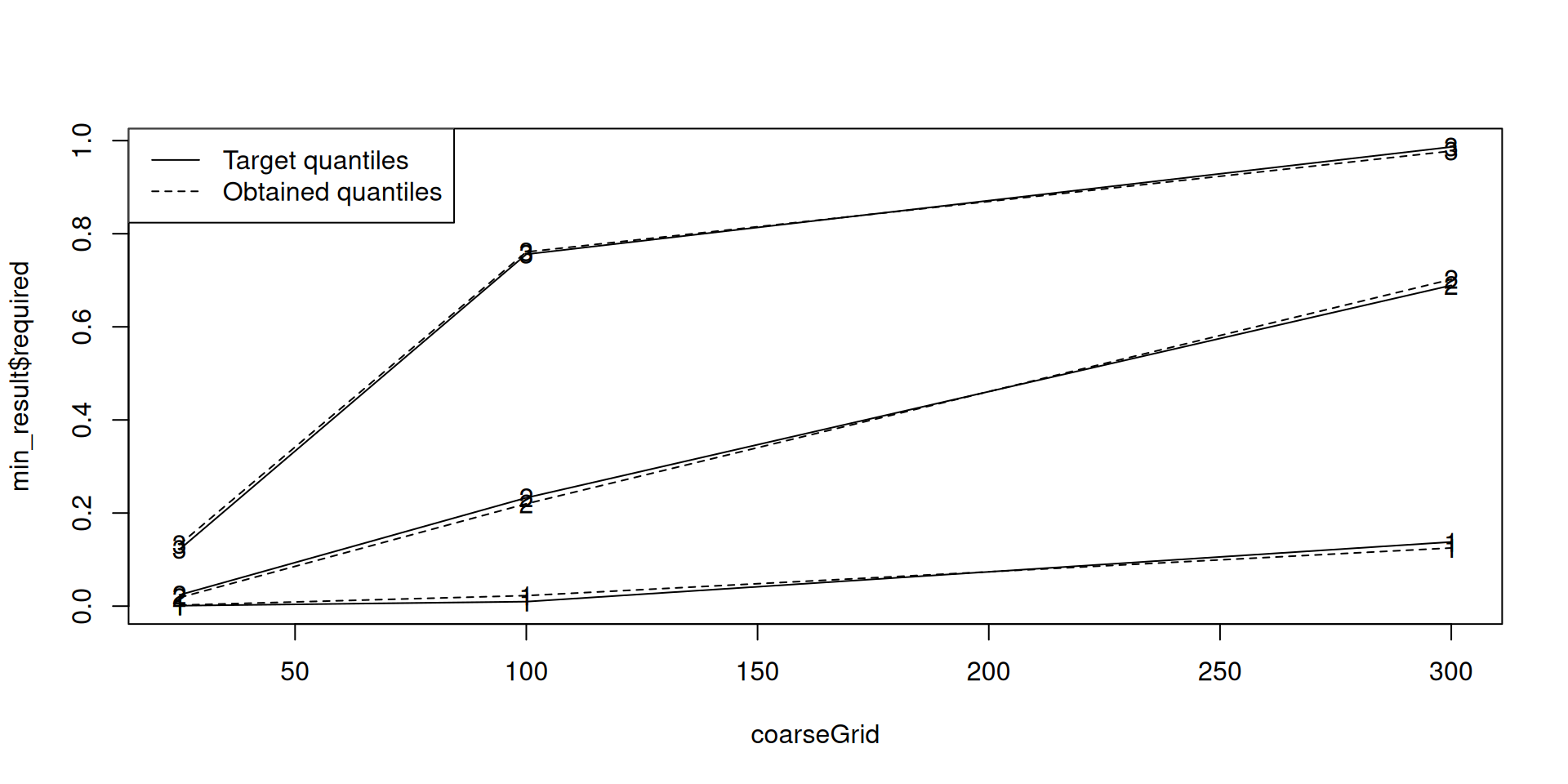
coarseGrid <- c(25, 100, 300)
min_result <- MinimalInformative(
  dosegrid = coarseGrid, 
  refDose = 100,
  logNormal = TRUE, # use a log-normal distribution for the slope parameter
  threshmin = 0.1, # the quantile for the low dose
  threshmax = 0.2, # the quantile for the high dose
  seed = 432, # for reproducibility
  control = list(max.time = 30) # limit the optimization time here
)

It: 1, obj value (lsEnd): 0.06732883077 indTrace: 1
It: 214, obj value (lsEnd): 0.01474025243 indTrace: 214
It: 238, obj value (lsEnd): 0.01416193999 indTrace: 238
It: 460, obj value (lsEnd): 0.01295269405 indTrace: 460
timeSpan = 30.000442 maxTime = 30
Emini is: 0.01295269405
xmini are:
-1.280026342 0.6618977116 1.254935046 0.1500300078 0.5608228116 
Totally it used 30.000481 secs
No. of function call is: 10147

Comparing the prior result with the target quantiles

matplot(
    x = coarseGrid,
    y = min_result$required,
    type = "o",
    lty = 1,
    col = 1
)
matlines(
    x = coarseGrid,
    y = min_result$quantiles,
    type = "o",
    lty = 2,
    col = 1
)
legend("topleft", legend = c("Target quantiles", "Obtained quantiles"), lty = 1:2, col = 1)

Comparing the prior result with the target quantiles

Resulting prior parameters

min_result$model

A logistic log normal model will describe the relationship between dose and toxicity: $$p(Tox | d) = f(X = 1 | \theta, d) = \frac{e^{\alpha + \beta \cdot log(d/d_{ref})}}{1 + e^{\alpha + \beta \cdot log(d/d_{ref})}}$$where d_ref denotes a reference dose.

The prior for θ is given by$$\boldsymbol\theta = \begin{bmatrix}\alpha \\ log(\beta)\end{bmatrix}\sim N \left(\begin{bmatrix}-1.28 \\ 0.66\end{bmatrix} , \begin{bmatrix} 1.57 & 0.11 \\ 0.11 & 0.02\end{bmatrix} \right)$$

The reference dose will be 100.00.

Mixture priors

• Sometimes we have more specific prior information about the toxicity probabilities at the doses of interest, for example from preclinical data or from similar drugs.
• In such cases, we can use mixture priors to incorporate this information into the CRM model
• For example, we can use a logistic log-normal model with a mixture of two normal distributions, with the weights of the two components reflecting our uncertainty about which scenario is more likely
• Applications of mixture priors include:
  • bimodal: e.g. one representing a “low toxicity” scenario and one representing a “high toxicity” scenario
  • borrowing from another compound: e.g. one representing the information from a similar drug and one representing a minimally informative prior
  • borrowing from another population: e.g. one representing the behavior from a global study population and one minimally informative

Mixture priors in crmPack

crmPack currently includes the following classes for mixture priors:

• LogisticNormalMixture:
  • standard logistic regression model with a mixture of $K=2$ bivariate normal priors on the intercept and slope parameters
  • the weight parameter is also estimated from the data and has a Beta hyperprior distribution
• LogisticNormalFixedMixture
  • standard logistic regression model with fixed mixture of multiple bivariate (log-) normal priors on the intercept and slope parameters
  • the weights are fixed, and $K>2$ mixture components can be used

Example of LogisticNormalMixture

Let’s first define two bivariate normal components:

comp1 <- ModelParamsNormal(
    mean = c(-0.85, 1),
    cov = matrix(c(1, -0.5, -0.5, 1), nrow = 2)
  )
comp2 <- ModelParamsNormal(
    mean = c(1, 1.5),
    cov = matrix(c(1.2, -0.45, -0.45, 0.6), nrow = 2)
  )

Say we use a uniform $\textrm{Beta}(1,1)$ hyperprior for the weight parameter, and a reference dose of $d^{*} = 50$:

normal_mix_prior <- LogisticNormalMixture(
    comp1 = comp1,
    comp2 = comp2,
    weightpar = c(a = 1, b = 1),
    ref_dose = 50
)
normal_mix_prior

A mixture of two logistic log normal models will describe the relationship between dose and toxicity: $$p(Tox | d) = f(X = 1 | \theta, d) = \frac{e^{\alpha + \beta \cdot log(d/d^*)}}{1 + e^{\alpha + \beta \cdot log(d/d^*)}}$$where d* denotes a reference dose.

The prior for θ is given by$$ \theta = \begin{bmatrix} \alpha \\ log(\beta) \end{bmatrix} \sim w \cdot The prior for θ is given by\n$$ = $$\begin{bmatrix}\alpha \\ \beta\end{bmatrix}$$ N ( $$\begin{bmatrix}-0.85 \\ 1.00\end{bmatrix}$$ , $$\begin{bmatrix} 1.00 & -0.50 \\ -0.50 & 1.00\end{bmatrix}$$

) $$

• (1 - w) The prior for θ is given by$$\boldsymbol\theta = \begin{bmatrix}\alpha \\ \beta\end{bmatrix}\sim N \left(\begin{bmatrix} 1.00 \\ 1.50\end{bmatrix} , \begin{bmatrix} 1.20 & -0.45 \\ -0.45 & 0.60\end{bmatrix} \right)$$

$$and the prior for w is given by

$$w \sim Beta(1, 1)$$The reference dose will be 50.00.

Example of LogisticNormalFixedMixture

Here we need to fix the weights of the mixture components, for example to 0.5 each:

normal_mix_fix_weights_prior <- LogisticNormalFixedMixture(
  components = list(
    comp1 = comp1,
    comp2 = comp2
  ),
  weights = c(0.5, 0.5),
    ref_dose = 50
)
normal_mix_fix_weights_prior

A mixture of 2 logistic log normal models with fixed weights will describe the relationship between dose and toxicity: $$p(Tox | d) = f(X = 1 | \theta, d) = \frac{e^{\alpha + \beta \cdot log(d/d^*)}}{1 + e^{\alpha + \beta \cdot log(d/d^*)}}$$where d* denotes a reference dose.

The prior for θ is given by$$\theta = \begin{bmatrix} \alpha \\ \beta \end{bmatrix} \sim \sum_{i=1}^{2}w_i \cdot N \left( \mathbf{\mu}_i , \mathbf{\Sigma}_i \right)$$ with $$\sum_{i=1}^{2} w_i = 1$$ The individual components of the mixture are $$\boldsymbol\theta_1 = \begin{bmatrix}\alpha \\ \beta\end{bmatrix}\sim N \left(\begin{bmatrix}-0.85 \\ 1.00\end{bmatrix} , \begin{bmatrix} 1.00 & -0.50 \\ -0.50 & 1.00\end{bmatrix} \right)$$

with weight 0.5 and $$\boldsymbol\theta_2 = \begin{bmatrix}\alpha \\ \beta\end{bmatrix}\sim N \left(\begin{bmatrix} 1.00 \\ 1.50\end{bmatrix} , \begin{bmatrix} 1.20 & -0.45 \\ -0.45 & 0.60\end{bmatrix} \right)$$

with weight 0.5 The reference dose will be 50.00.

Comparison of the two prior specifications

We can easily see the difference in the JAGS code:

body(normal_mix_prior@priormodel)

{
    w ~ dbeta(weightpar[1], weightpar[2])
    wc <- 1 - w
    comp0 ~ dbern(wc)
    comp <- comp0 + 1
    theta ~ dmnorm(mean[1:2, comp], prec[1:2, 1:2, comp])
    alpha0 <- theta[1]
    alpha1 <- theta[2]
}

body(normal_mix_fix_weights_prior@priormodel)

{
    comp ~ dcat(weights)
    theta ~ dmnorm(mean[1:2, comp], prec[1:2, 1:2, comp])
    alpha0 <- theta[1]
    alpha1 <- theta[2]
}

Yet another but different mixture prior

• LogisticLogNormalMixture
  • standard logistic model with online mixture of $K=2$ bivariate log normal priors on the intercept and slope parameters
  • can be used when data is arising online from the informative component of the prior, at the same time with the data of the trial of main interest
  • assumes the same prior distribution for the informative component and the current trial data (for simplicity), the only question is whether the parameters are identical or not
  • needs to use DataMixture class to specify the data structure for the online data

Example of LogisticLogNormalMixture

Note that we just use one component, i.e. one prior here:

online_mix_prior <- LogisticLogNormalMixture(
    share_weight = 0.5, # probability that the current and external data are from the same distribution
    ref_dose = 50,
    mean = comp1@mean,
    cov = comp1@cov
)

Now we define the data, which consists of the current trial data and the external data:

data_share <- DataMixture(
    doseGrid = c(25, 50, 100, 200, 300),
    x = c(25, 25, 50, 50),
    y = c(0, 1, 0, 1),
    xshare = c(25, 25, 50, 50, 100, 100, 300, 300),
    yshare = c(0, 0, 0, 1, 0, 0, 0, 1)
)

Example of LogisticLogNormalMixture (cont’d)

Let’s look at the model definition:

body(online_mix_prior@priormodel)

{
    for (k in 1:2) {
        theta[k, 1:2] ~ dmnorm(mean, prec)
        alpha0[k] <- theta[k, 1]
        alpha1[k] <- exp(theta[k, 2])
    }
    comp ~ dcat(cat_probs)
}

body(online_mix_prior@datamodel)

{
    for (i in 1:nObs) {
        stand_log_dose[i] <- log(x[i]/ref_dose)
        logit(p[i]) <- alpha0[comp] + alpha1[comp] * stand_log_dose[i]
        y[i] ~ dbern(p[i])
    }
    for (j in 1:nObsshare) {
        stand_log_dose_share[j] <- log(xshare[j]/ref_dose)
        logit(pshare[j]) <- alpha0[2] + alpha1[2] * stand_log_dose_share[j]
        yshare[j] ~ dbern(pshare[j])
    }
}

We see that comp == 2 means that the current and external data are from the same distribution, while comp == 1 means they are from different distributions.

Example of LogisticLogNormalMixture (cont’d)

We can produce samples then as usually:

samples_share <- mcmc(data_share, online_mix_prior, McmcOptions())
plot(samples_share, online_mix_prior, data_share)

Probability that the current and external data are from the same distribution:

mean(samples_share@data$comp == 2)

[1] 0.5825

References

Neuenschwander, B, M Branson, and T Gsponer. 2008. “Critical Aspects of the Bayesian Approach to Phase i Cancer Trials.” Statistics in Medicine.