crmPack Training for Merck

Basic Training

Daniel Sabanés Bové

RPACT

March 31, 2026

Basic Training Outline 📦

• Motivation
• Model-based dose escalation design
• Example study design
• Calculating operating characteristics
• Backfilling cohorts

Acknowledgements

Part of this training material is based on the crmPack training materials developed by John Kirkpatrick (Roche, now at Astellas). Thanks John for sharing!

Motivation

Maximum tolerated dose (MTD)

• The main purpose of a First-in-Human (FIH) study is usually to define the Maximum Tolerated Dose (MTD) of the IMP
• Usually, the MTD is defined in terms of the highest acceptable incidence of Dose-Limiting Toxicities (DLTs) at a given dose
• The definition of a DLT varies with indication and may vary from the serious (life-threatening SAEs) to the innocuous (mild headache)

Overview of dose escalation designs

• Rule-based designs: 3+3 (Lin and Shih 2015), accelerated titration, rolling 6 (Skolnik et al. 2008), etc.
• Model-based designs: Continual Reassessment Method (CRM) (O’Quigley et al. 1990), Escalation with Overdose Control (EWOC) (Neuenschwander et al. 2008), etc.
• Model-assisted designs: mTPI (Ji et al. 2010), Keyboard, Bayesian Optimal Interval (BOIN) (Liu and Yuan 2015), etc.

3+3 design

Figure taken from “Principles of dose finding studies in cancer: A comparison of trial designs”

3+3 vs. model-based designs

	3+3	CRM
Definition of a DLT	Study specific	Study specific
The target toxicity rate	0.33	Any
The dose grid	Study specific	Study specific
The cohort size	3	Any
The stopping rule(s)	2 DLTs at same dose	Any
The eligibility rule	One dose up	Any
The escalation rule	+1 if 0/3 or 1/6	Any
The definition of the MTD	Max dose with <2 DLTs	Any
The dose-toxicity model	None	Any

Higher-level overview

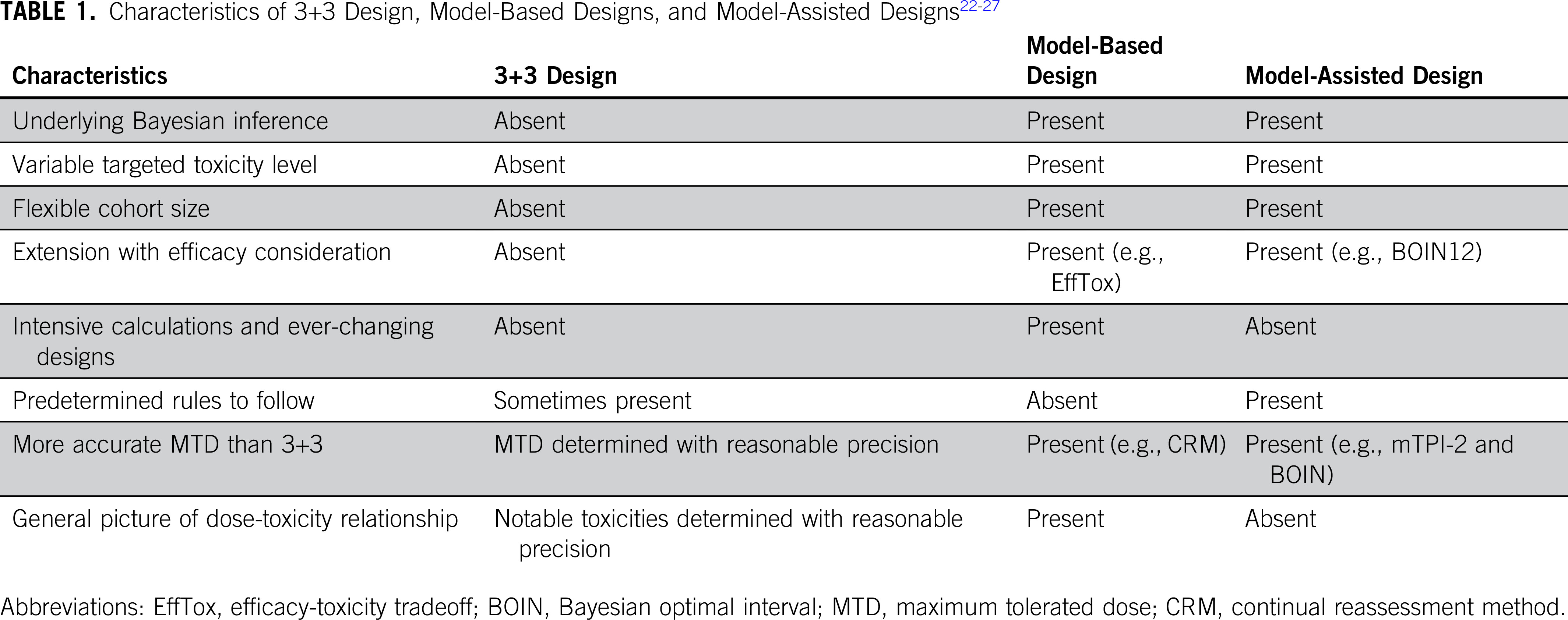
Table taken from “Moving Beyond 3+3: The Future of Clinical Trial Design”

Usage of model-based designs

• Rogatko et al. (2007) reported that 98.4% of phase I cancer trials use a 3+3 design or a variant, but that only 35% of participants is such trials were treated at “optimal” doses, compared to 55% in model-based trials
• Le Tourneau et al. (2009) reported 3.3% (6 of 181) of trials used CRM during 2007–2008
• van Brummelen et al. (2016) reported that only 6.4% (11 of 172 oncology Phase I trials) used model-based approaches from 2012 to 2014
• Nonami et al. (2025) reported that from 394 clinical trials submitted to PMDA between 2013 and 2022, 195 (49.5%) used rule-based designs, 114 (28.9%) used model-based designs and 85 (21.6%) used model-assisted designs.

crmPack to the rescue!

With crmPack we aim to make it easy for everyone to use model-based designs in their dose escalation studies. The package provides:

• A flexible framework to define dose escalation designs
• Calculation of operating characteristics via simulations
• Visualization and tabulation of results
• A user-friendly interface to backfill cohorts
• A growing collection of advanced design options (e.g. dual endpoint designs, time-to-event designs, etc.)

Model-based dose escalation design

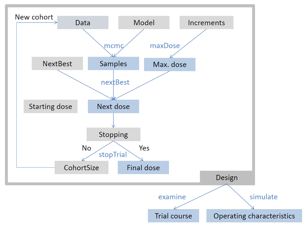
Flow chart

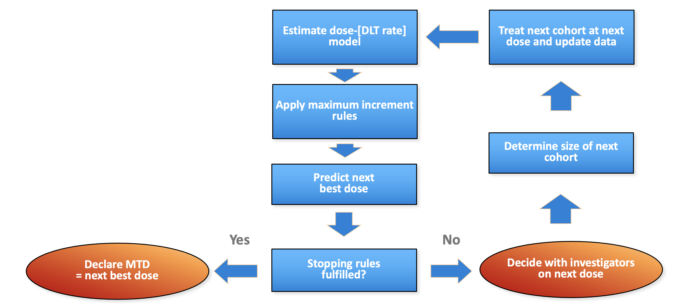
Generic flow chart for model-based dose escalation design

Package structure: parallel to flow

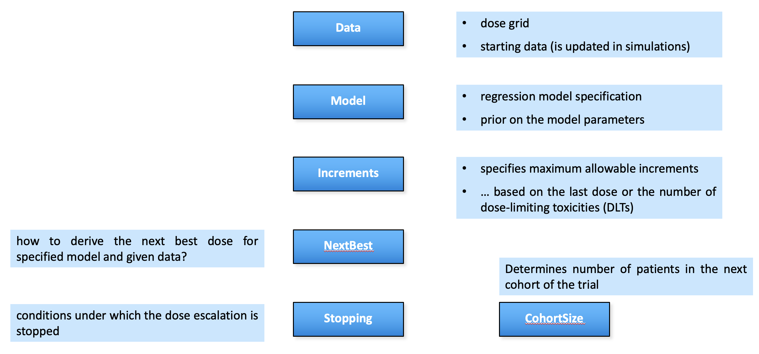
crmPack package structure parallels the flow chart

Framework in crmPack

crmPack package framework

Example study design

Data object

We first need to decide what the possible doses could be, i.e. the so-called dose grid:

library(crmPack)

dose_grid <- c(1, 5, seq(from = 10, to = 200, by = 1))

This we use to initialize our (still empty, i.e. without patients) Data object, which will be used to store the data of our trial as it progresses:

empty_data <- Data(doseGrid = dose_grid)

Adding a patient

We can “update” the Data object with the information of a patient treated at dose 10, who did not experience a DLT, and a patient at dose 20 with a DLT:

data <- empty_data |> 
    update(x = 10, y = 0) |> 
    update(x = 20, y = 1)

And plot it:

plot(data)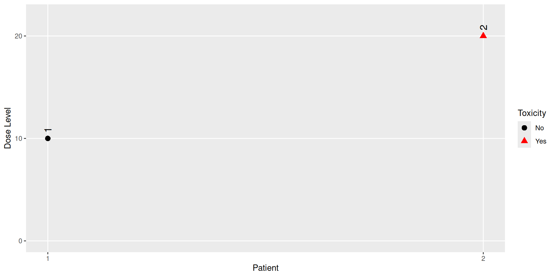

Model object

Next we need to specify the dose-toxicity model we want to use.

Often used is this logistic model with reference dose $d_{ref}$, which assigns the following probability of DLT to a dose $x$:

$$\mathbb{P}(Y = 1 | x) = \frac{e^{\alpha + \beta \cdot log(x / d_{ref})}}{1 + e^{\alpha + \beta \cdot log(x / d_{ref})}}$$

Then we also use a prior distribution for the parameters $\alpha$ and $\beta$. Typically, we want $\beta$ to be positive, so we can assign a bivariate normal distribution to $(\alpha, \log(\beta))$.

Model object (cont’d)

For example, let’s use the following model:

get_cov <- function(sigma0, sigma1, rho) {
  matrix(c(sigma0^2, rho * sigma0 * sigma1, rho * sigma0 * sigma1, sigma1^2), nrow = 2)
}
model <- LogisticLogNormal(
  mean = c(-3, 0.5),
  cov = get_cov(sigma0 = 1, sigma1 = 2, rho = 0.5),
  ref_dose = 20
)

Model object (cont’d)

In Quarto/Rmarkdown, we will get the nice textual description of the model by just printing it:

model

A logistic log normal model will describe the relationship between dose and toxicity: $$p(Tox | d) = f(X = 1 | \theta, d) = \frac{e^{\alpha + \beta \cdot log(d/d_{ref})}}{1 + e^{\alpha + \beta \cdot log(d/d_{ref})}}$$where d_ref denotes a reference dose.

The prior for θ is given by$$\boldsymbol\theta = \begin{bmatrix}\alpha \\ log(\beta)\end{bmatrix}\sim N \left(\begin{bmatrix}-3.00 \\ 0.50\end{bmatrix} , \begin{bmatrix} 1.00 & 1.00 \\ 1.00 & 4.00\end{bmatrix} \right)$$

The reference dose will be 20.00.

Generating prior and posterior samples

We use MCMC, in particular Gibbs sampling implemented in JAGS, to generate (approximate) samples from the posterior distribution of the model parameters. The settings are controlled by the McmcOptions object. Note that in order to get reproducible results, we also need to set the random seed:

mcmc_options <- McmcOptions(
  burnin = 1000,
  step = 10,
  samples = 1000,
  rng_kind = "Mersenne-Twister",
  rng_seed = 12345
)

Now we can generate the prior and posterior samples with the mcmc method:

prior_samples <- mcmc(model, data = empty_data, options = mcmc_options)
posterior_samples <- mcmc(model, data = data, options = mcmc_options)

MCMC settings recommendations

• The default MCMC settings are:
  • burn-in: 10,000
  • step: 2
  • samples: 10,000
• We just saw that we can use lower numbers during development
• Also the more complex the model, the longer the MCMC chain should be run
• The most important is to check the convergence of the MCMC chain:

names(posterior_samples@data)

[1] "alpha0" "alpha1"

alpha0_samples <- get(posterior_samples, "alpha0")
library(ggmcmc)
ggs_traceplot(alpha0_samples)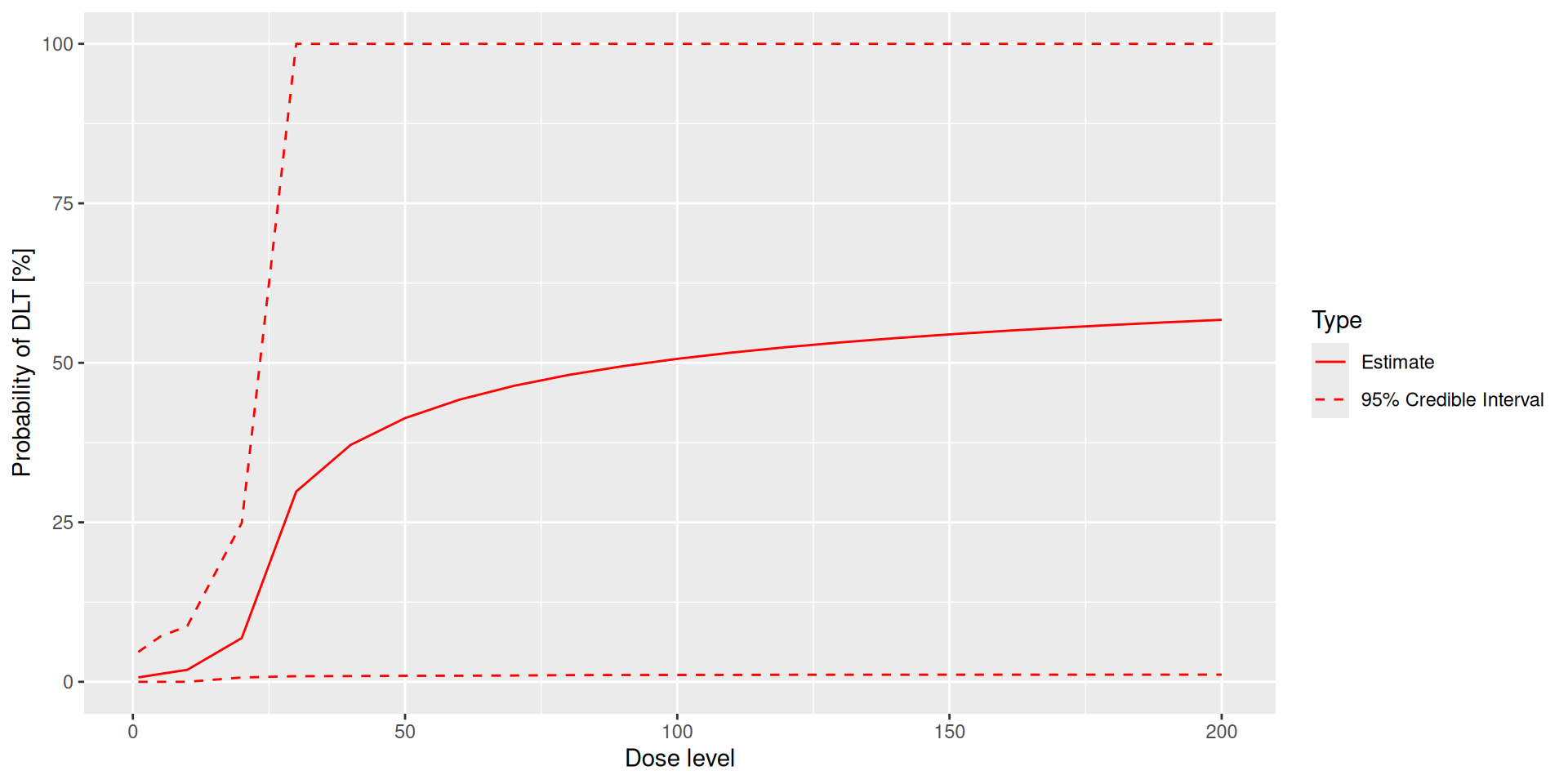

ggs_autocorrelation(alpha0_samples)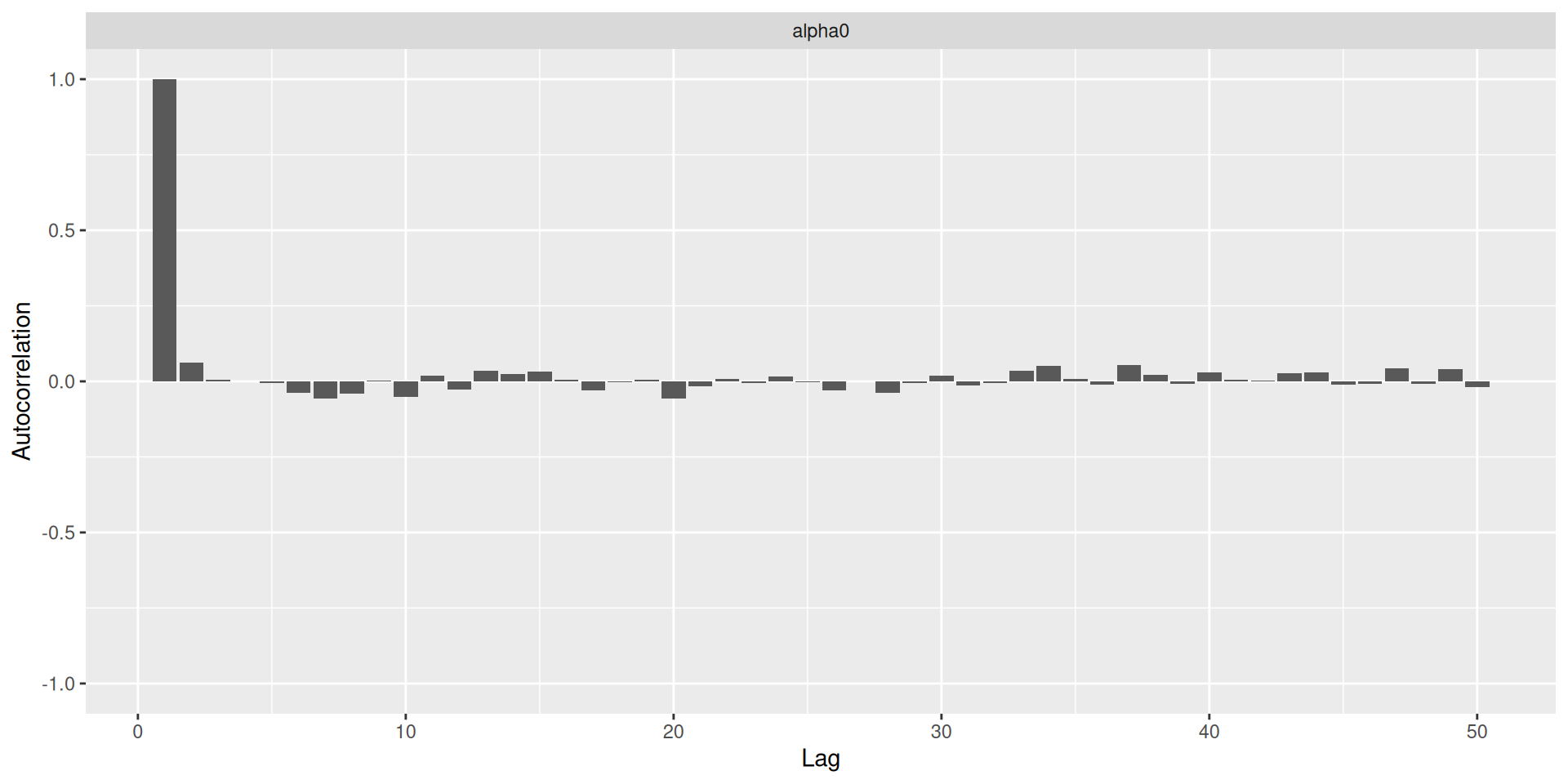

Plotting dose-toxicity curves: Prior

plot(prior_samples, model, empty_data)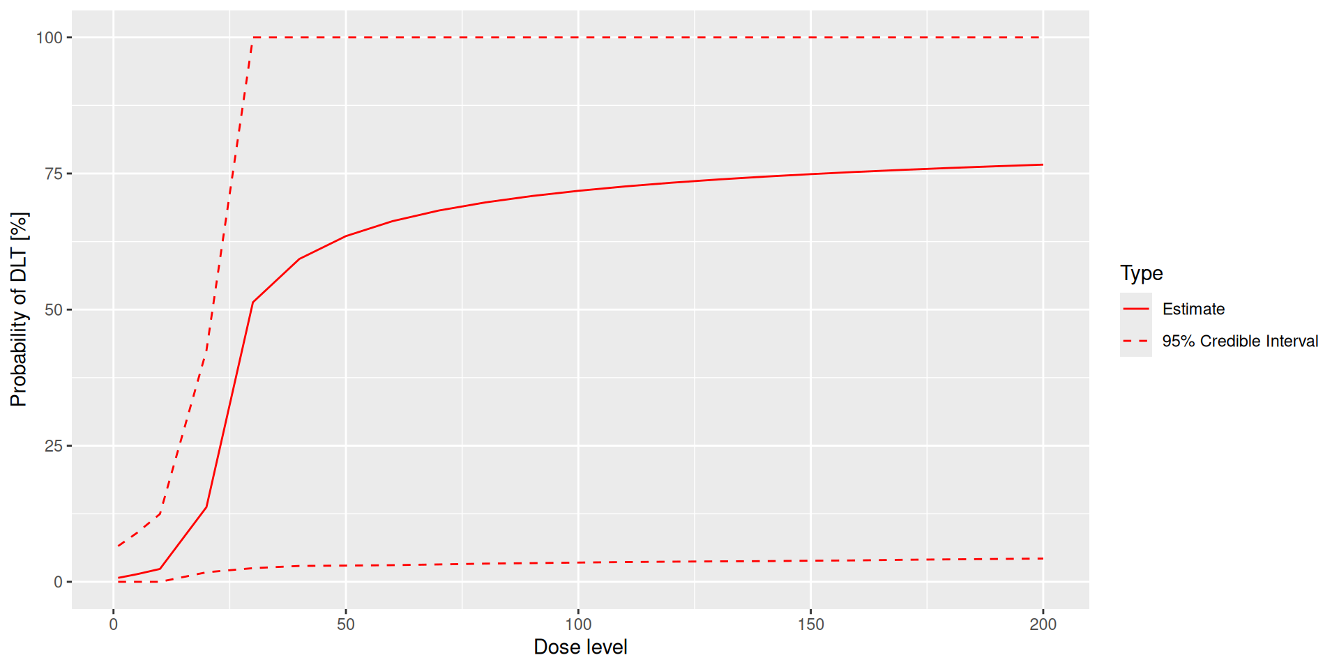

Plotting dose-toxicity curves: Posterior

plot(posterior_samples, model, data)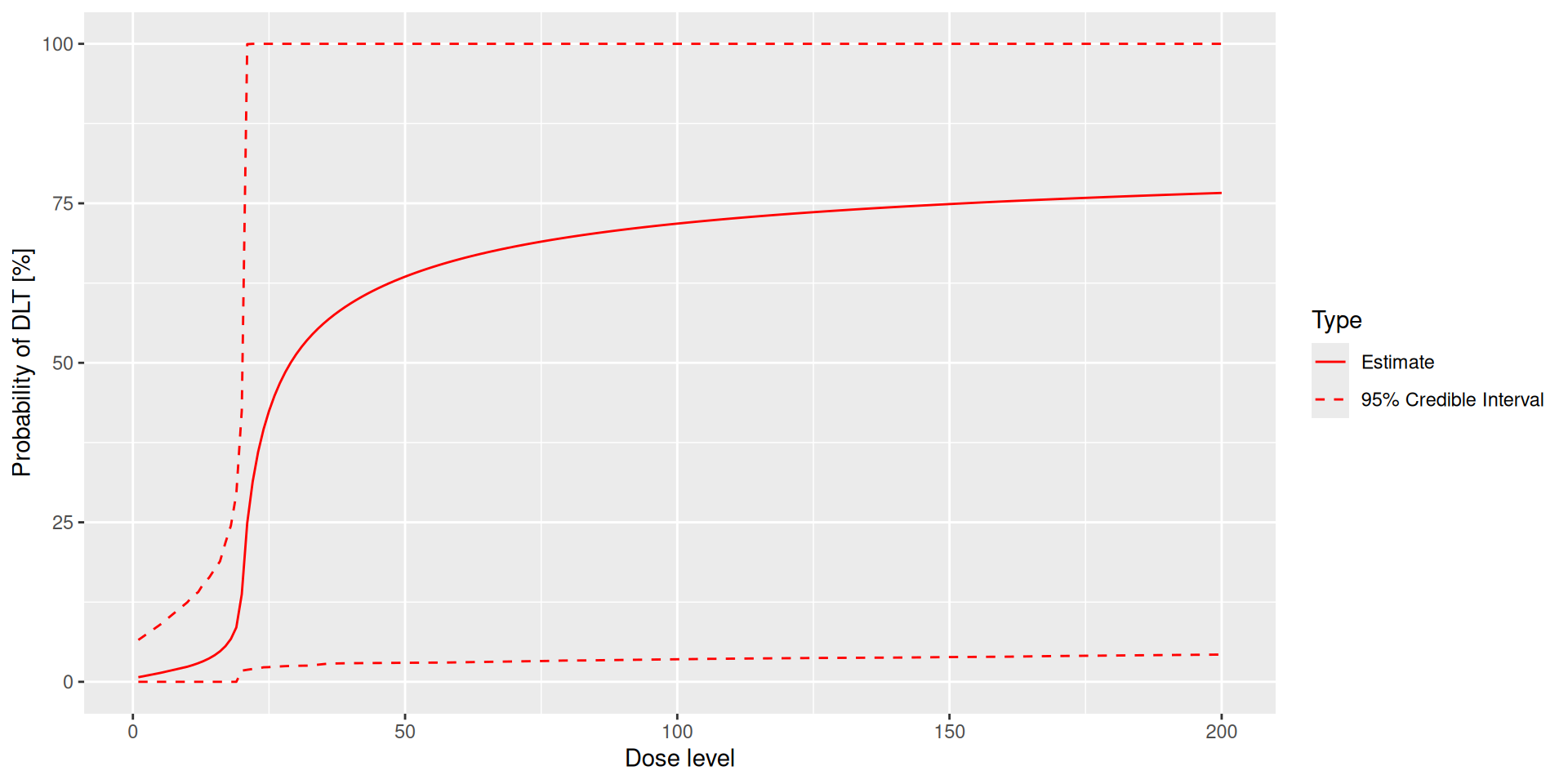

Increments object

We usually need additional safety rules for our model-based dose escalation design. For example, we might restrict the maximum allowed dose increment to 100% (i.e. doubling the dose) if no DLTs have been observed, and to 50% if one DLT has been observed. This can be implemented with an Increments object:

increments <- IncrementsRelativeDLT(
    intervals = c(0, 1),
    increments = c(1, 0.5)
)
increments

Defined by number of DLTs reported so far

No DLTs
Min	Max	Increment
0	1	1.0
1	Inf	0.5

NextBest object

Together with the regression model, the definition of how to obtain the recommendation for the dose of the next cohort, are the key components of the model-based dose escalation design.

For example, we can minimize the posterior expected loss while restricting the maximum overdosing (e.g. 40-100% DLTs) probability to less than 25%:

next_best <- NextBestNCRMLoss(
    target = c(0.2, 0.4), # loss: 0
    overdose = c(0.4, 0.7), # loss: 1
    unacceptable = c(0.7, 1), # loss: 2
    max_overdose_prob = 0.25,
    losses = c(1, 0, 1, 2) # underdosing has loss 1
)
next_best

The dose recommended for the next cohort will be chosen in the following way:

• First, the chance that the probability of toxicity falls into each of the underdose, target , overdose and unacceptable dose ranges is calculated for element of the dose grid.
• Next, the loss associated with each dose is calculated by multiplying these probabilities by the corresponding loss coefficient and summing the result.
• Then ineligible doses, and those with a probability of being in the overdose or unaccaptable ranges that is greater than 0.25, are discarded.
• Finally, the dose level with the smallest loss is selected as the recommended dose for the next cohort.

Toxicity ranges and loss coefficients are given in the following table:

Range	Lower	Upper	Loss Coefficient
Underdose	0.0	0.2	1
Target	0.2	0.4	0
Overdose	0.4	0.7	1
Unacceptable	0.7	1.0	2

CohortSize object

In the simplest case, we just always have the same constant number of patients in each cohort, e.g. 3 patients per cohort:

cohort_size <- CohortSizeConst(3)

As with all components, other options are available, see ?CohortSize for details.

Stopping object

Typically there are stopping rules for a dose escalation study. In the simplest case, this is just the number of patients treated, e.g. 30 patients:

stop1 <- StoppingMinPatients(nPatients = 30)

But we can also combine this with logical & and | operators with other stopping rules, e.g. to also stop if the target probability is high, or if the model would not recommend any dose at all because of safety concerns:

stop2 <- StoppingTargetProb(target = c(0.2, 0.3), prob = 0.7)
stop3 <- StoppingMissingDose()
stopping <- stop1 | stop2 | stop3
stopping

If any of the following rules are TRUE:

• ≥ 30 patients dosed: If 30 or more participants have been treated.

• P(0.2 ≤ prob(DLE | NBD) ≤ 0.3) ≥ 0.7: If the probability of toxicity at the next best dose is in the range [0.20, 0.30] is at least 0.70.

• Stopped because of missing dose: If the dose returned by nextBest() is NA, or if the trial includes a placebo dose, the placebo dose.

Resulting recommendation example

So in our data example from above, what would be the recommended dose for the next cohort?

First, the maximum increment is calculated using the maxDose method:

max_dose <- maxDose(increments, data)
max_dose

[1] 30

Here it is only 30, because we observed one DLT at dose 20, so the maximum allowed increment is 50%.

Then the next best dose is calculated with the nextBest method:

next_best_dose <- nextBest(
  next_best, 
  doselimit = max_dose, 
  samples = posterior_samples, 
  model = model, 
  data = data
)

Resulting recommendation example (cont’d)

The joint plot is in the $plot_joint element of the result (target/overdose/unacceptable probabilities and expected loss for each dose):

print(next_best_dose$plot_joint)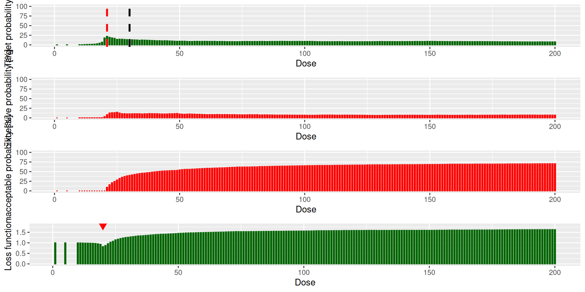

And the value is in the $value element:

next_best_dose$value

[1] 20

So due to the high probability of overdosing at dose 30, the recommended dose for the next cohort is dose 20, which is the same as the previous cohort.

Resulting recommendation example (cont’d)

We can also use the fit() method to get the posterior quantiles, and we can combine that with the loss results to get a nice table:

fitted_df <- fit(posterior_samples, model, data)
loss_df <- next_best_dose$probs |> as.data.frame() |> dplyr::select(dose, posterior_loss)
result_df <- dplyr::left_join(fitted_df, loss_df, by = "dose") 
knitr::kable(head(result_df), digits = 3)

dose	middle	lower	upper	posterior_loss
1	0.007	0	0.066	0.999
5	0.014	0	0.090	0.998
10	0.024	0	0.125	0.996
11	0.026	0	0.135	0.995
12	0.029	0	0.141	0.991
13	0.033	0	0.154	0.988

Operating characteristics

Design object

First we need to put all the components of our model-based dose escalation design together in a Design object - here we also need to define a starting dose:

design <- Design(
    data = empty_data,
    model = model,
    nextBest = next_best,
    increments = increments,
    cohort_size = cohort_size,
    stopping = stopping,
    startingDose = 5
)
design

Design

Dose toxicity model

A logistic log normal model will describe the relationship between dose and toxicity: $$p(Tox | d) = f(X = 1 | \theta, d) = \frac{e^{\alpha + \beta \cdot log(d/d_{ref})}}{1 + e^{\alpha + \beta \cdot log(d/d_{ref})}}$$where d_ref denotes a reference dose.

The prior for θ is given by$$\boldsymbol\theta = \begin{bmatrix}\alpha \\ log(\beta)\end{bmatrix}\sim N \left(\begin{bmatrix}-3.00 \\ 0.50\end{bmatrix} , \begin{bmatrix} 1.00 & 1.00 \\ 1.00 & 4.00\end{bmatrix} \right)$$

The reference dose will be 20.00.

Stopping rule

If any of the following rules are TRUE:

• ≥ 30 patients dosed: If 30 or more participants have been treated.

• P(0.2 ≤ prob(DLE | NBD) ≤ 0.3) ≥ 0.7: If the probability of toxicity at the next best dose is in the range [0.20, 0.30] is at least 0.70.

• Stopped because of missing dose: If the dose returned by nextBest() is NA, or if the trial includes a placebo dose, the placebo dose.

Escalation rule

Defined by number of DLTs reported so far

No DLTs
Min	Max	Increment
0	1	1.0
1	Inf	0.5

Use of placebo

Placebo will not be administered in the trial.

Backfill cohorts

No backfill cohorts at all will be opened.

Dose recommendation

The dose recommended for the next cohort will be chosen in the following way:

• First, the chance that the probability of toxicity falls into each of the underdose, target , overdose and unacceptable dose ranges is calculated for element of the dose grid.
• Next, the loss associated with each dose is calculated by multiplying these probabilities by the corresponding loss coefficient and summing the result.
• Then ineligible doses, and those with a probability of being in the overdose or unaccaptable ranges that is greater than 0.25, are discarded.
• Finally, the dose level with the smallest loss is selected as the recommended dose for the next cohort.

Toxicity ranges and loss coefficients are given in the following table:

Range	Lower	Upper	Loss Coefficient
Underdose	0.0	0.2	1
Target	0.2	0.4	0
Overdose	0.4	0.7	1
Unacceptable	0.7	1.0	2

Cohort size

A constant size of 3 participants.

Observed data

No participants are yet evaluable.

The dose grid is 1, 5, 10, 11, 12, 13, 14, 15, 16, 17, 18, 19, 20, 21, 22, 23, 24, 25, 26, 27, 28, 29, 30, 31, 32, 33, 34, 35, 36, 37, 38, 39, 40, 41, 42, 43, 44, 45, 46, 47, 48, 49, 50, 51, 52, 53, 54, 55, 56, 57, 58, 59, 60, 61, 62, 63, 64, 65, 66, 67, 68, 69, 70, 71, 72, 73, 74, 75, 76, 77, 78, 79, 80, 81, 82, 83, 84, 85, 86, 87, 88, 89, 90, 91, 92, 93, 94, 95, 96, 97, 98, 99, 100, 101, 102, 103, 104, 105, 106, 107, 108, 109, 110, 111, 112, 113, 114, 115, 116, 117, 118, 119, 120, 121, 122, 123, 124, 125, 126, 127, 128, 129, 130, 131, 132, 133, 134, 135, 136, 137, 138, 139, 140, 141, 142, 143, 144, 145, 146, 147, 148, 149, 150, 151, 152, 153, 154, 155, 156, 157, 158, 159, 160, 161, 162, 163, 164, 165, 166, 167, 168, 169, 170, 171, 172, 173, 174, 175, 176, 177, 178, 179, 180, 181, 182, 183, 184, 185, 186, 187, 188, 189, 190, 191, 192, 193, 194, 195, 196, 197, 198, 199 and 200.

Starting dose

The starting dose is 5.

Examine method

The first “quick check” we should run on our design is how it behaves if we don’t see any DLTs at all - can we even reach the higher doses? This can be done with the examine method:

examine(design)

   dose DLTs nextDose  stop increment
1     5    0       10 FALSE       100
2     5    1        5 FALSE         0
3     5    2        5 FALSE         0
4     5    3        5 FALSE         0
5    10    0       20 FALSE       100
6    10    1       15 FALSE        50
7    10    2       15 FALSE        50
8    10    3       15 FALSE        50
9    20    0       20 FALSE         0
10   20    1       20 FALSE         0
11   20    2       20 FALSE         0
12   20    3       19 FALSE        -5
13   20    0       21 FALSE         5
14   20    1       21 FALSE         5
15   20    2       20 FALSE         0
16   20    3       20 FALSE         0
17   21    0       23 FALSE        10
18   21    1       21 FALSE         0
19   21    2       20 FALSE        -5
20   21    3       20 FALSE        -5
21   23    0       26 FALSE        13
22   23    1       23 FALSE         0
23   23    2       22 FALSE        -4
24   23    3       21 FALSE        -9
25   26    0       31 FALSE        19
26   26    1       26 FALSE         0
27   26    2       24 FALSE        -8
28   26    3       22 FALSE       -15
29   31    0       41 FALSE        32
30   31    1       31 FALSE         0
31   31    2       28 FALSE       -10
32   31    3       26 FALSE       -16
33   41    0       82 FALSE       100
34   41    1       46 FALSE        12
35   41    2       34 FALSE       -17
36   41    3       30 FALSE       -27
37   82    0      153  TRUE        87
38   82    1       77  TRUE        -6
39   82    2       54  TRUE       -34
40   82    3       42  TRUE       -49

Here it could be also concerning that if we observe 3 DLTs at the starting dose of 5, we still continue with the same dose 5 for the next cohort. The reason here is that the prior is “too confident” that at low doses we have a low DLT probability.

Adjusted performance

So we need to adjust the prior to be less confident, e.g. by changing the means and the standard deviations of the parameters, changing the reference dose, and checking the plot:

model_adjusted <- LogisticLogNormal(
  mean = c(-3, -1),
  cov = get_cov(sigma0 = 4, sigma1 = 1, rho = 0),
  ref_dose = 100
)
prior_samples_adjusted <- mcmc(model_adjusted, data = empty_data, options = mcmc_options)
plot(prior_samples_adjusted, model_adjusted, empty_data)

design_adjusted <- design
design_adjusted@model <- model_adjusted
examine(design_adjusted)

   dose DLTs nextDose  stop increment
1     5    0       10 FALSE       100
2     5    1        1 FALSE       -80
3     5    2       NA  TRUE        NA
4     5    3       NA  TRUE        NA
5    10    0       19 FALSE        90
6    10    1       15 FALSE        50
7    10    2        5 FALSE       -50
8    10    3        1 FALSE       -90
9    19    0       37 FALSE        95
10   19    1       28 FALSE        47
11   19    2       17 FALSE       -11
12   19    3       10 FALSE       -47
13   37    0       61 FALSE        65
14   37    1       51 FALSE        38
15   37    2       31 FALSE       -16
16   37    3       22 FALSE       -41
17   61    0      122 FALSE       100
18   61    1       90 FALSE        48
19   61    2       50 FALSE       -18
20   61    3       38 FALSE       -38
21  122    0      189 FALSE        55
22  122    1      128 FALSE         5
23  122    2       97 FALSE       -20
24  122    3       70 FALSE       -43
25  189    0      197 FALSE         4
26  189    1      200 FALSE         6
27  189    2      154 FALSE       -19
28  189    3      122 FALSE       -35
29  197    0      195 FALSE        -1
30  197    1      200 FALSE         2
31  197    2      199 FALSE         1
32  197    3      172 FALSE       -13
33  195    0      180 FALSE        -8
34  195    1      200 FALSE         3
35  195    2      199 FALSE         2
36  195    3      200 FALSE         3
37  180    0      181  TRUE         1
38  180    1      200  TRUE        11
39  180    2      200  TRUE        11
40  180    3      200  TRUE        11

Toxicity scenarios

In order to evaluate the operating characteristics of our design, we need to define some toxicity scenarios, i.e. the true dose-toxicity relationship in the population. This needs to be a function mapping a dose vector to a vector of DLT probabilities. This could be:

• Logistic curve
• Probit curve
• Power curve
• Manual specification of DLT probabilities at each dose level

For example:

scenario1 <- function(x) {
    plogis(- 2 + 0.8 * log(x / 20))
}

Toxicity scenarios (cont’d)

curve(scenario1, from = 1, to = 200, ylim = c(0, 1))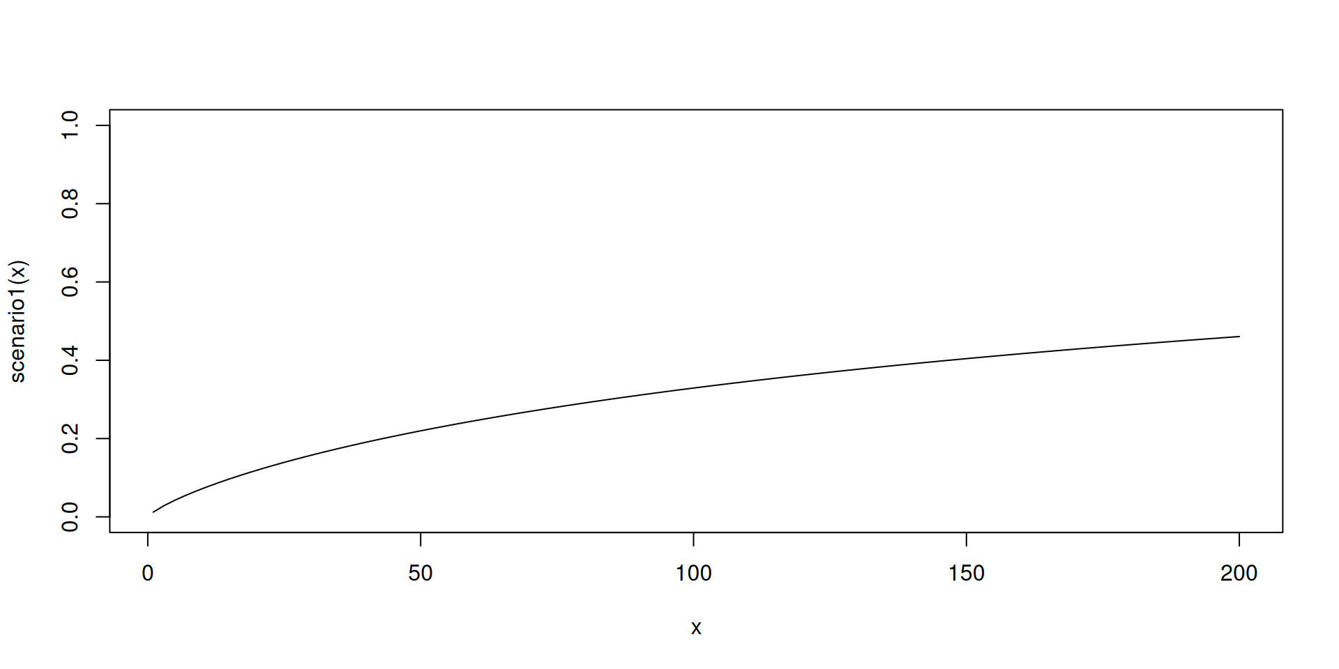

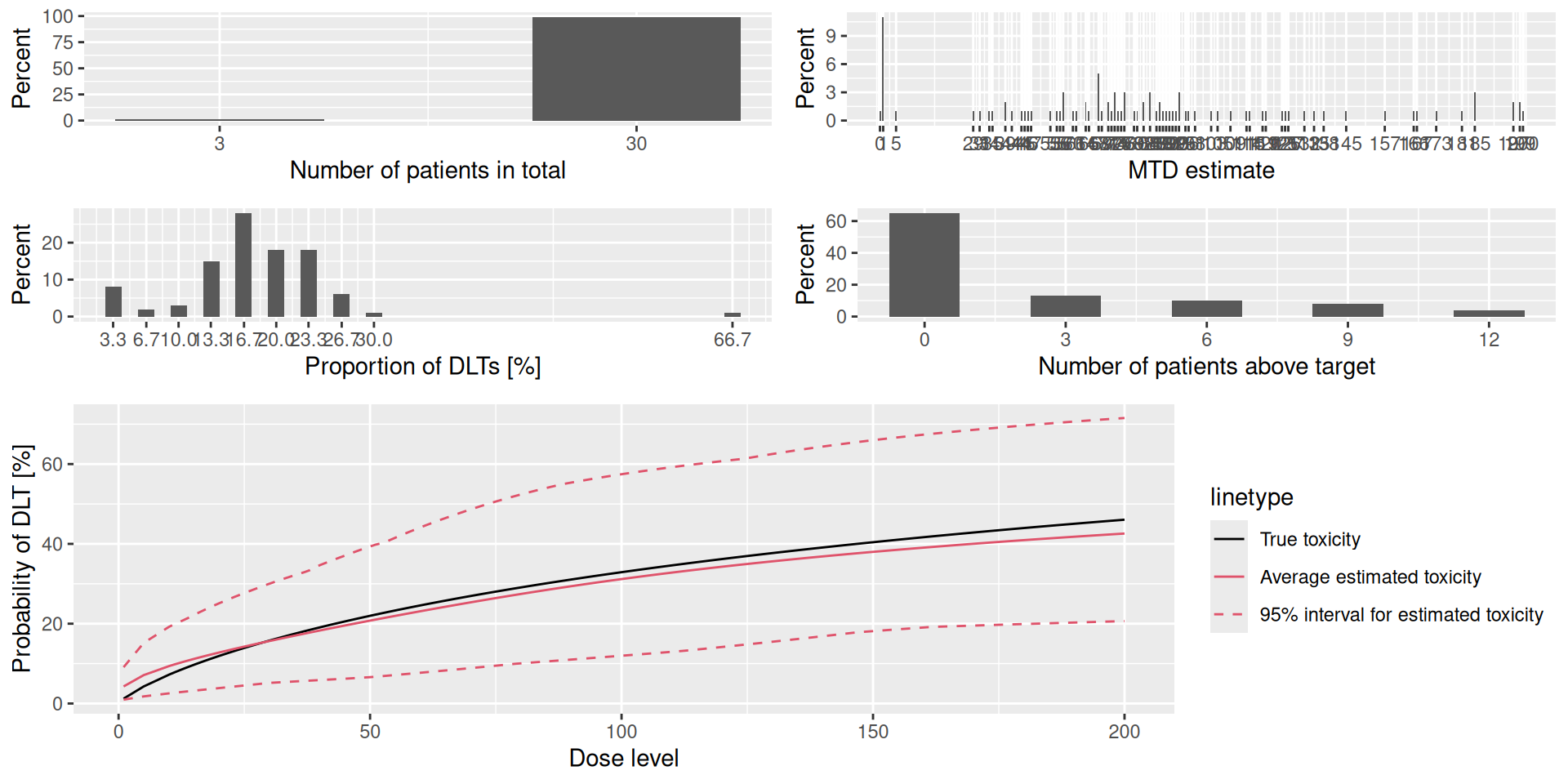
Running simulations

Now given the design and the toxicity scenario, we can run simulations with the simulate method:

sims <- simulate(
    design_adjusted,
    nsim = 100,
    truth = scenario1,
    mcmcOptions = mcmc_options,
    seed = 123,
    parallel = TRUE
)

Backfilling cohorts

Especially in oncology trials, it is meanwhile common to open backfill cohorts at lower dose levels while the escalation cohorts are still ongoing at higher dose levels. Recently this was implemented in crmPack with the Backfill objects.

For example:

backfill_simple <- Backfill(
  cohort_size = CohortSizeConst(3),
  max_size = 12,
  opening = OpeningMinCohorts(min_cohorts = 1),
  recruitment = RecruitmentUnlimited(),
  priority = "lowest"
)
backfill_simple

Cohort size: A constant size of 3 participants.

Opening rule: If 1 or more cohorts have been treated in total.

Recruitment: Unlimited recruitment of backfill patients is allowed.

Total number of backfill patients: 12 backfill patients.

Priority of higher vs. lower dose backfill cohorts: lowest dose.

Backfilling cohorts (cont’d)

This can then be added in the corresponding backfill slot of the Design object:

design_backfill <- design_adjusted
design_backfill@backfill <- backfill_simple

Please note that the examine method does not yet take the backfilling into account, so it will still show the same results as before. To see the effect of the backfilling, we need to run simulations.

Summarizing results

We can get basic summaries of the simulation results with the summary method:

sims_summary <- summary(sims, truth = scenario1)
sims_summary

Summary of 100 simulations

Target toxicity interval was 20, 35 %
Target dose interval corresponding to this was 43.1, 112.4 
Intervals are corresponding to 10 and 90 % quantiles

Number of patients overall : mean 30 (30, 30) 
Number of patients treated above target tox interval : mean 2 (0, 9) 
Proportions of DLTs in the trials : mean 18 % (10 %, 23 %) 
Mean toxicity risks for the patients on active : mean 18 % (2 %, 24 %) 
Doses selected as MTD : mean 82.7 (1, 167.6) 
True toxicity at doses selected : mean 27 % (1 %, 43 %) 
Proportion of trials selecting target MTD: 56 %
Dose most often selected as MTD: 1 
Observed toxicity rate at dose most often selected: 2 %
Fitted toxicity rate at dose most often selected : mean 4 % (2 %, 7 %) 
Stop reason triggered:
 ≥ 30 patients dosed :  99 %
 P(0.2 ≤ prob(DLE | NBD) ≤ 0.3) ≥ 0.7 :  0 %
 Stopped because of missing dose :  1 %

Plotting results

And we can also get more detailed plots of the simulation results with the plot method:

plot(sims)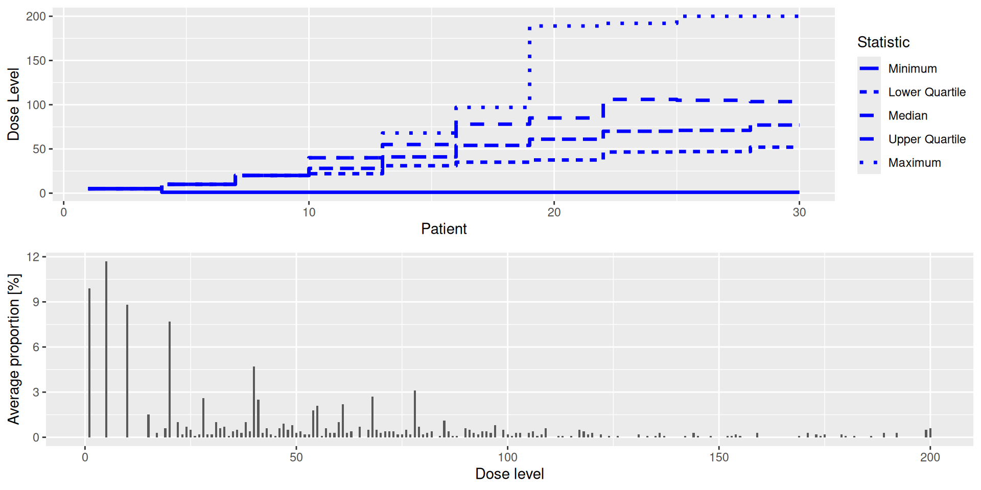

Plotting results (cont’d)

The summary result can also be plotted:

plot(sims_summary)

Learning more

Learning more

Lots of documentation is available on the crmPack website: crmPack.org

It includes:

• 13 vignettes with detailed examples of how to use the package
  • In particular, the paper vignette is a great starting point
  • Also backfilling cohorts are explained in a dedicated backfilling vignette e.g.
• Link to the online reference explaining all the functions and classes in the package
• Contact information for questions and suggestions, as well as a link to the GitHub repository for bug reports and feature requests

References

Ji, Y, P Liu, Y Li, and N Bekele. 2010. “A Modified Toxicity Probability Interval Method for Dose-Finding Trials.” Clin Trials 7: 653–63. https://doi.org/doi.org/10.1177/1740774510382799.

Le Tourneau, C, JJ Lee, and LL Siu. 2009. “Dose Escalation Methods in Phase i Cancer Clinical Trials.” J Natl Cancer Inst, 708–20.

Lin, Y, and WJ Shih. 2015. “Statistical Properties of the Traditional Algorithm-Based Designs for Phase i Cancer Clinical Trials.” Biostatistics 2: 203 -- 215. https://doi.org/doi.org/10.1093/biostatistics/2.2.203.

Liu, S, and Y Yuan. 2015. “Bayesian Optimal Interval Designs for Phase i Clinical Trials.” JRSS(C) 64: 507 -- 523.

Neuenschwander, B, M Branson, and T Gsponer. 2008. “Critical Aspects of the Bayesian Approach to Phase i Cancer Trials.” Statistics in Medicine.

Nonami, Atsushi, Kensuke Matsuda, Kouta Funakoshi, Ryosuke Kato, Hideaki Takahashi, and Yoko Edahiro. 2025. “Impact of Dose-Escalation Design on the Safety and Development of Anticancer Drugs in Clinical Trials.” Clinical and Translational Science 18 (10): e70367. https://doi.org/https://doi.org/10.1111/cts.70367.

O’Quigley, John, Margaret Pepe, and Lloyd Fisher. 1990. “Continual Reassessment Method: A Practical Design for Phase 1 Clinical Trials in Cancer.” Biometrics 46 (1): 33–48.

Rogatko, A, D Shoeneck, W Jonas, M Tighiouart, FR Khuri, and A Porter. 2007. “Translation of Innovative Designs into Phase 1 Trials.” J Clin Onc 25 (31): 4982–86.

Skolnik, JM, JS Barrett, B Jayaraman, D Patel, and PC Adamson. 2008. “Shortening the Timeline of Pediatric Phase i Trials: The Rolling Six Design.” J Clin Onc 26 (2): 190–95. https://doi.org/10.1200/JCO.2007.12.7712.

van Brummelen, EM, AD Huitema, E van Werkhoven, JH Beijnen, and JH Schellens. 2016. “The Performance of Model-Based Versus Rule-Based Phase i Clinical Trials in Oncology: A Quantitative Comparison of the Performance of Model-Based Versus Rule-Based Phase i Trials with Molecularly Targeted Anticancer Drugs over the Last 2 Years.” J Pharmacokinet Pharmacodyn 43 (3): 235–42.